Unconventional U.S. onshore drilling has risen in recent years due to the technological combination of horizontal drilling and hydraulic fracturing. Together, these processes are recognized as capable of unearthing considerable assets of oil and natural gas in areas once thought less productive. In the past, the Tuscaloosa Marine Shale (TMS) Play has proven to produce both oil and gas, and the likelihood of opportunities extending past Louisiana and Mississippi into the Eagle Ford Basin located in Texas is high.
Together, TGS and Beicip Inc. have created nonexclusive basin temperature cubes and fluid composition, maturity and pressure distribution models of the TMS that go beyond the resistivity control of the play. It is believed that by having multiple layers of information on prospectivity, it will enhance exploration and development of the TMS play by understanding and encouraging expansion using factors that directly impact production such as pressure, viscosity and phase.
Why the TMS?
The TMS, which covers millions of acres in southern Louisiana and parts of western Mississippi, is of similar geological age as its neighboring basin the Eagle Ford. The TMS is divided into three major formation layers: Upper Tuscaloosa (Eagle Ford-Tuscaloosa), which is comprised of sands and shales; Tuscaloosa Marine Shale, which includes the elevated resistivity zone; and the Lower Tuscaloosa (Woodbine) consisting of argillaceous sands.
The primary zone of interest varies in thickness throughout the play, ranging from 152.4 m (500 ft) to more than 244 m (800 ft) within an area from 3,049 m to 4,573 m (10,000 ft to 15,000 ft) deep. Permeability ranges from less than 0.1 mD to 0.06 mD, while porosity varies from 2.3% to 8%. In the 1997 Bulletin from the Basin Research Institute the TMS was estimated to have reserves of about 7 Bbbl of oil in a 15,281-sq-km (5,900-sq-mile) area.
BTM
A new methodology for basin temperature modeling (BTM) has been developed that uses large volumes of properly indexed and quality-controlled (QCd) bottomhole temperature (BHT) data for onshore basins or areas. This method honors the observation that borehole temperatures equilibrate, increasing toward formation temperature with elapsed time since fluid circulation (TSC).
The maximum BHTs recorded in a layer (normalized for depth) or cell are used rather than a corrected average or regression-based model. This type of temperature modeling can be used to identify where favorable gas-to-oil ratios (GORs) exist for shale gas formations. Lithostratigraphic units (with common lithologies) have an interval geothermal gradient that can be significantly different from their overlying and underlying units and can vary with depth.
Therefore, the interval temperature gradient needs to be determined based on depth and lithology. The TMS thermal study consisted of 9,500 QCd BHT points with valid TSC from 4,172 wells, with layering based on tops picked in 1,491 wells totaling 18 tops. Key wells that were representative of the basin and composed of good well log curve responses were used for picking tops. A total of four 3-D temperature volumes were constructed for the TMS, all illustrating different views of the thermal variations within the basin (Figure 1).
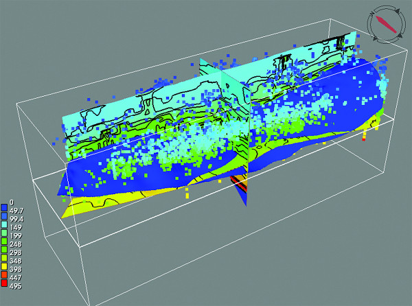
FIGURE 1. The MaxBHT volume was used in BTM in the TMS. (Source: TGS)
TOC calculation
Several intervals were analyzed to create organic-rich thickness maps. According to the stratigraphy, the Eagle Ford equivalent can be divided into three members in the vicinity of the study: TMS, the Woodbine and the Upper Tuscaloosa/Eagle Ford. Each one of these maps was computed using the CARBOLOG (carbon organic log) method developed by the Institut Francais du Petrole using more than 300 wells.
This analytic method exploits the physical properties of the organic matters, which are characterized by high sonic transit time and by a high resistivity (Carpentier et al., 1991). The result can be analyzed in a 1/ √Rt ∆T plot. This method is calibrated using four distinct pure component poles: water, organic matter, clay and matrix. These poles are calibrated following the compaction trend rule, environmental deposition settings and values from publication.
The results were used as input for the fluid-flow modeling to better estimate the geographical presence of organic matter in the system. It also brought new hypotheses and questions in both known and unknown areas. It is possible to add proprietary data such as laboratory data to enhance the results and provide a map of reconstructed total organic carbon (TOC) instead of an organic-rich thickness map.

FIGURE 2. The play can be expanded using geological and thermal attributes. (Source: Beicip)
GOR prediction
The basin temperature data and model are integrated using basinwide calibration points, and the temperature is propagated from basin inception to present day using an advanced thermal basement module. This takes into account the heat transfer from deep earth (asthenosphere) through the mechanical layers of the earth (lithosphere) and into the base of sediments.
The heat is then propagated using thermal properties of sedimentary rocks such as conductivities, heat capacity and radiogenic heat production for certain rock, particularly for radioactive shales. Burial history of sedimentary rocks is reconstructed within the thermal model to compute maturity of the TMS.
Consequently, a first major result is obtained with regard to hydrocarbon fluid quality: black oil, volatile oil, wet-gas and dry-gas windows. Once maturity modeling is completed, a compositional forward model is computed for organic matter cracking into oil, gas and late gas, which allows calculation of GORs throughout the model. E&P companies can use these results to explore new areas beyond the current play boundaries and into deeper intervals as well as new counties and parishes (Figure 2).
Pressure analysis
Unconventional resource production from nonreservoir formations with very low permeability-to-viscosity ratios that require permeability-creating mechanisms (Cander, 2012) such as fracking need special attention to not only understand and predict the fluid composition of the hydrocarbons to extract but also track phase behavior at changing formation pressures.
Bubble point and dew point computation become critical to predicting phase evolution with pressure drop inherent to hydrocarbon production. In this study, thermal maturity and pressure were examined to predict GOR distribution over the TMS in Louisiana, Mississippi and East Texas, first as a function of thermal maturity and then as a function of organofacies variations. Saturation pressure is calculated using a basin-scale compositional fluid-flow model, and head room pressure is deduced.
In the experiment from Hoshkiw (1970), the effect of pressure on oil and gas in contact is illustrated using different values of pressure. Temperature is kept constant. The BeicipFranlab-TGS study aimed at predicting the saturation pressure below which free gas comes out of solution and results in production complications. The goal is to calculate the difference in pressure between stages 6 and 4.
Understanding when Stage 4 is reached during production is key. Using this kind of analysis, combined with bringing proprietary data for pressure and geometry at a very local scale, production companies can implement developments in advance. Having this type of information can aid in distinguishing how long and up to what pressure companies can continue producing before inducing phase separation and production complications (Figure 3).

FIGURE 3. Head room pressure can be predicted to determine GOR. Using this kind of analysis, production companies can implement developments in advance. (Source: Beicip)