Whether it’s conventional EOR or hydraulic fracturing, one of the key questions operators ask is where is the injected fluid going in the subsurface? Far-field resistivity mapping answers those questions. Resistivity, long a standard in wireline logging for detecting hydrocarbons, can also be used to detect tertiary recovery flood fronts—CO2, water, steam, etc. Hydraulic fracture fluids also can be mapped to define the extent of fluid invasion. This information, combined with an operator’s knowledge of the field or formation, yields direct answers to optimize field development.
Methodology
GroundMetrics’ method depends upon two key field components. First is the eQube capacitive sensor. This technology was first deployed by the U.S. Department of Defense. It has been repackaged with new workflows specifically designed to answer oilfield questions. Unlike porous pot-type galvanic sensors, the eQube needs simply to be in contact with the ground surface. It does not need to be buried, nor does it require constant wetting with an agent to assure electrical coupling. Moreover, as capacitive sensors do not rely upon chemical/ion exchange for coupling, reliability and repeatability are greatly increased. Ease of use speeds deployment and minimizes maintenance requirements during a project.
The construction and specialized feedback circuits contained in the sensor assure a broadband response from 0.01 Hz to greater than 500 Hz. Tests have demonstrated that the sensor is more sensitive than traditional porous pot sensors without the requirement of burial or specialized muds.
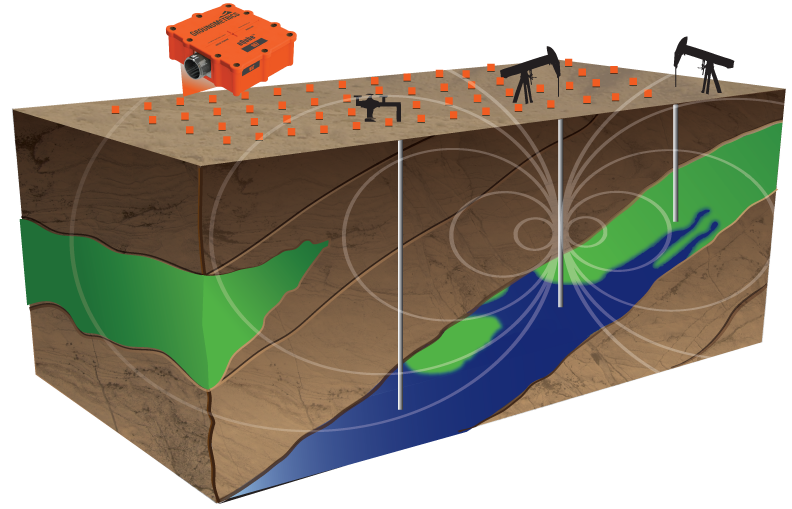
Second, surface resistivity measurements on land are well known to have rather shallow depth of penetration. To assure signal returning to the surface array, GroundMetrics uses a local wellbore as an antenna. The transmitter can be connected to the wellhead, or an electrode can be lowered into a wellbore via wireline. This technique greatly improves transmission signal at the formation of interest (Figure 1).
The data are collected over a few days continuously. They are processed to produce an anomaly map to yield a plan view of change in resistivity. Optionally, an inversion can be applied to produce a volumetric representation of the resistive anomaly.
Waterflood application
The client in this case had encountered a series of dry holes (Figure 2). The questions posed were:
- Where is the water relative to the well(s) and fault?
- Is there room for another well in the up-thrown reservoir?
- Can we determine the fault location?
- Can we see the oil/water contact?
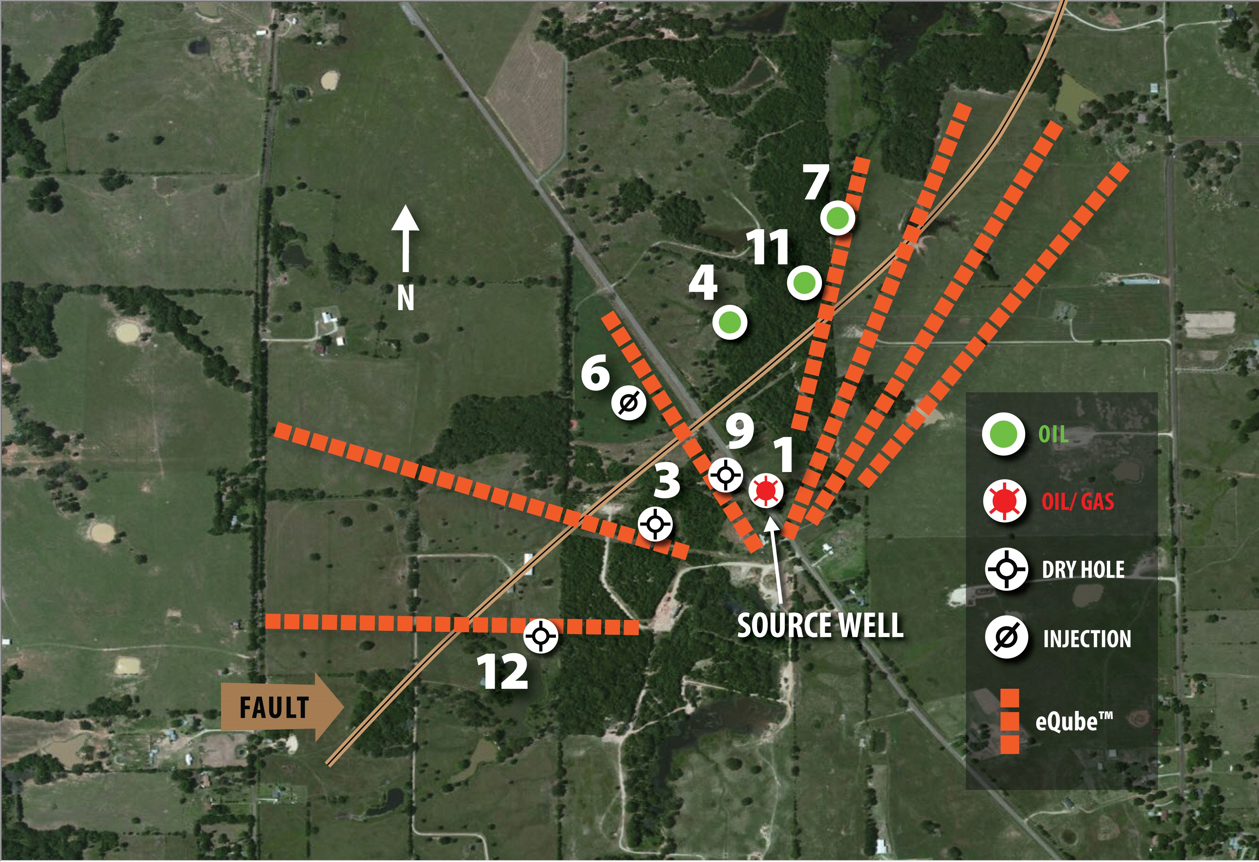
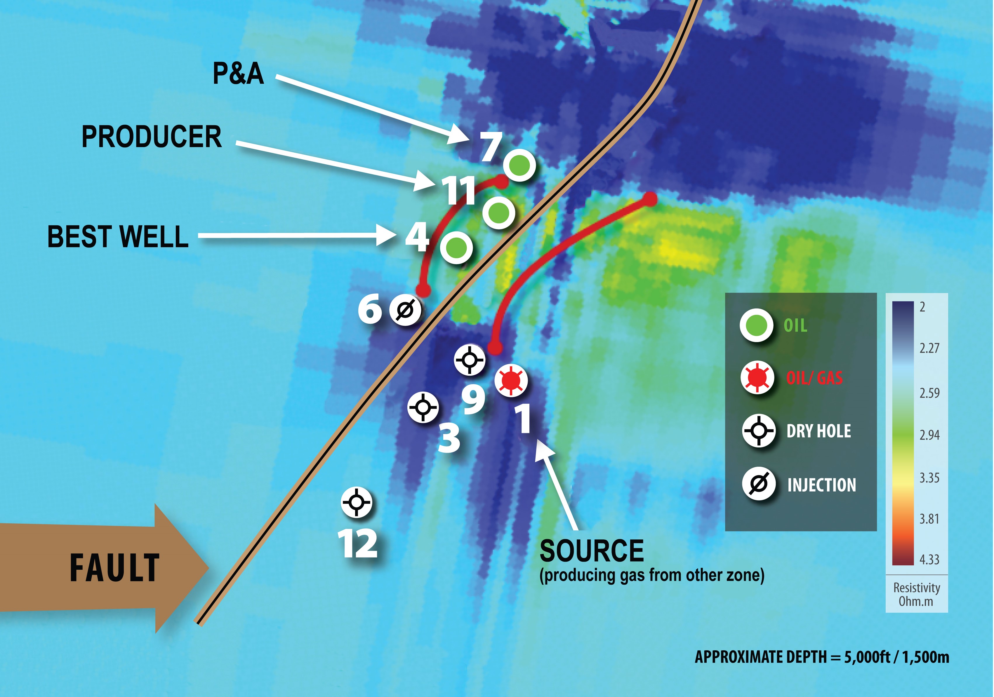
GroundMetrics performed a survey and processed the data through inversion. The result is shown in Figure 3. In Figure 2, the producers are Wells 4, 11 and 7 on the up-thrown side of a fault. Wells 3, 9 and 12, drilled on the down-thrown side of the fault, were dry. Well 2 produced some oil and gas. Well 6 is the water injector for this field. The lines of orange squares indicate where the sensors were deployed. Well 1 was used as the transmission antenna. Figure 3 displays the resultant resistivity contrasts after inversion. The warmer colors are higher resistivity contrast, and the cooler colors are lower. With the resistivity data, the client’s questions can be answered. First, the producing accumulation is a stratigraphic trap on the up-thrown side. Well 7 was drilled very near the oil/water contact in the northeast. Wells 3, 9 and 12 are clearly off of the anomaly and in the water. 4 and 11 are centered on the resistive anomaly. Well 1 is also very close to the oil/water contact on the south side. On the up-thrown side there is no room for additional wells. For completeness, the large anomaly east of the fault is on a competitor’s acreage. Had the surface resistivity data been available, several dry holes could have been avoided.
Hydraulic fracturing
In this case the question posed was whether the sensor technology could detect the injection of fluid during hydraulic fracturing operations. Compared to a water or CO2 flood, the volumes used in hydraulic fracturing are much smaller. It is here the sensitivity of the sensor really becomes advantageous.
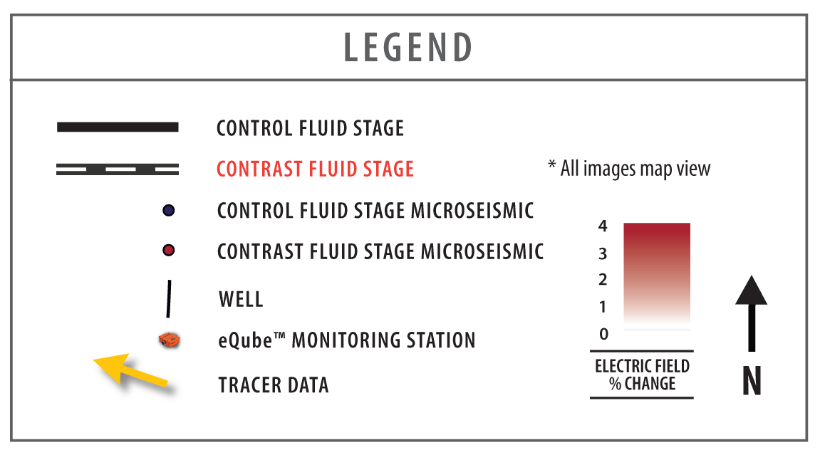
The project was in the Denver-Julesburg Basin in Colorado. Seven stages were monitored over several days. Four of the stages were pumped using a control fluid, commonly used in fracking. Three were pumped using a contrast fluid, a slightly different fluid commonly used in fracking, to produce an electromagnetic contrast. Figure 4 shows the setup for the experiment. An electrode on a wireline was pumped to a point in Well 8 adjacent to the treatment Well 7. Monitoring stations were placed over the area of interest. In addition to the GroundMetrics technology, surface microseismic, borehole microseismic and tracers were used in this test.

Figure 5 is the final resistivity difference map over the area of interest after all pumping on the seven stages was complete. The treatment Well 7 is the second well from the right on the map. The solid lines indicate the stages that were pumped with control fluid, and the dashed lines are the stages with contrast fluid. Note first that the two contrast fluid stages to the south in Well 7 show significantly higher resistivity contrast as indicated by the more intense red color of the resistivity data compared to adjacent control fluid stages. However, the final contrast fluid stage (Stage 5) does not indicate the same higher resistivity contrast. In fact, it appears that the resistivity contrast has been displaced to the west and south, suggesting that the fluid rapidly migrated during the stage. The included microseismic data support this interpretation. The blue circles are microseismic data detected during the pumping of the control fluid stages, and the red events correspond to microseismic data detected during the contrast fluid stages. Note in particular that the red microseismic data seem to indicate fluid movement to the west as well. The tracer injected in the final contrast fluid stage was detected in Well 5, two wells west of the treatment Well 7. This confirms the resistivity data. Fluid from Well 7 did traverse across the pad to the west and intersect Well 5. GroundMetrics also delivers a movie volume for projects that benefit from time-lapse display such as in this frack monitoring case. This volume can be formatted for most interpretive or visualization platforms.

Both for conventional EOR and hydraulic fracturing applications, this technology adds additional useful information to understand how the formation of interest is responding to injected fluid.
Acknowledgment
The author wishes to acknowledge Encana and Dr. H. Frank Morrison of Berkeley Geophysics Associates for their participation in and support of this project.
Some of this material is based upon work supported by the Department of Energy.
References available.
Recommended Reading

TGS, SLB to Conduct Engagement Phase 5 in GoM
2024-02-05 - TGS and SLB’s seventh program within the joint venture involves the acquisition of 157 Outer Continental Shelf blocks.
StimStixx, Hunting Titan Partner on Well Perforation, Acidizing
2024-02-07 - The strategic partnership between StimStixx Technologies and Hunting Titan will increase well treatments and reduce costs, the companies said.
Forum Energy Signs MOU to Develop Electric ROV Thrusters
2024-03-13 - The electric thrusters for ROV systems will undergo extensive tests by Forum Energy Technologies and SAFEEN Survey & Subsea Services.
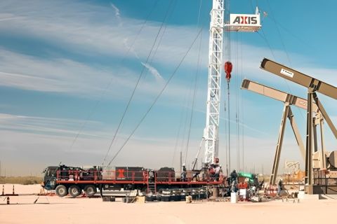
Axis Energy Deploys Fully Electric Well Service Rig
2024-03-13 - Axis Energy Services’ EPIC RIG has the ability to run on grid power for reduced emissions and increased fuel flexibility.

TotalEnergies Rolling Out Copilot for Microsoft 365
2024-02-27 - TotalEnergies’ rollout is part of the company’s digital transformation and is intended to help employees solve problems more efficiently.