
(Source: Eddytb Foto/Shutterstock.com)
[Editor's note: A version of this story appears in the August 2020 edition of E&P. Subscribe to the magazine here.]
Geology is 3D and needs to be represented in three dimensions to provide better reservoir understanding. With depths of investigation in the region of 100 ft to 150 ft, 3D inversion of data from the EarthStar ultradeep electromagnetic (EM) tool allows reservoir complexities to be represented in all directions at distances that allow early well placement decisions and well planning of subsequent wells in 3D.
The EarthStar ultradeep resistivity service is an LWD technology that helps operators map reservoir and fluid boundaries more than 200 ft from the wellbore using 1D inversion, more than doubling the depth of investigation of current industry offerings. The service delivers a comprehensive reservoir view so operators can eliminate costly pilot holes and sidetracks, make informed geosteering decisions in real time and better plan future field development.
As a part of the Earthstar service, a 3D reservoir mapping capability provides a more detailed representation of subsurface structures to improve well placement in complex reservoirs out to a depth of 150 ft. 3D inversion reveals overlooked features such as faults, water zones or local structural Nigel Clegg, Halliburton variations that can considerably alter the optimal placement of a well.
Historically, 1D inversion of ultradeep EM data has been deployed in many complex reservoirs to understand reservoir morphology and the position of fluids within the reservoir. Curtain plot displays show the distribution of multiple reservoir boundaries plotted directly above and below the wellbore. Identification of resistivity boundaries distant from the wellbore allows changes to the position of formation and fluid boundaries to be identified early, and well paths to be modified to achieve optimal well placement.
The extreme depths of investigation possible with these tools also allow secondary targets to be identified and subsequent wells to be planned to target them, increasing the success rate and providing cost savings. The 1D approach assumes that geology is a layer cake and formations are continuous to the sides of the wellbore; in fact, geology is 3D, with the potential for change to formations and fluids in all directions.
A 3D problem requires a 3D solution to allow assessment of a reservoir in all directions and allow well placement decisions to be made that involve changes in well azimuth as well as inclination to place the well in the most productive reservoir zones.
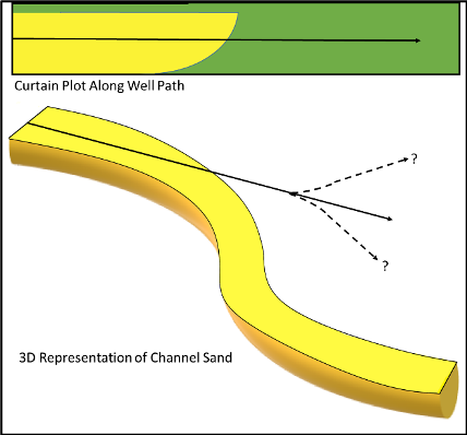
along the well path is represented in the top image. 1D inversion would display the position of resistivity bodies in this way. A 3D representation of a channel sand is depicted in the bottom image; the curtain plot sliced along the well path would not show the lateral migration of the channel. (Source: Halliburton)
3D geology
The importance of a 3D understanding of the reservoir can be demonstrated with a relatively simple and common reservoir target: channel sands (Figure 1).
Where a well exits a channel, a 1D inversion will only display the position of the upper and lower boundaries. It is not evident from which side of the channel that the well has exited or if the channel has just pinched out. It might be possible with other image tools to identify how the well exited the sand, but there is high uncertainty as to the position or continued existence of the channel. This scenario can be represented with a simple model and inverted using the 3D algorithm to show the benefit of assessing a reservoir in 3D (Figure 2).
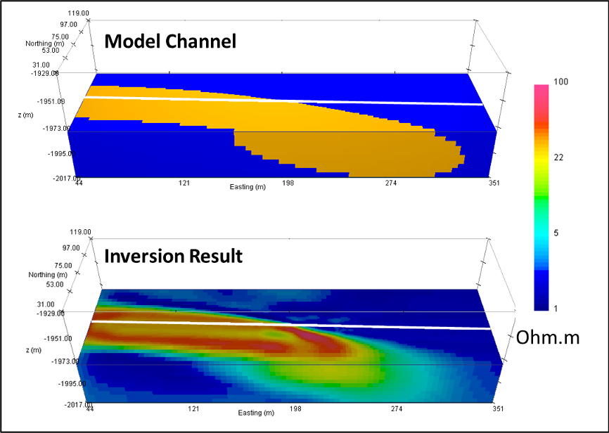
Not only is it clear how the well has exited the target sand channel, but it is also clear before the well exits the channel that it is approaching the side of the channel. Changes to the well azimuth could prevent the exit from the target if this is acted on early enough.
3D inversion process
The 3D inversion employs a deterministic algorithm to produce a single model that represents the distribution of resistivities around the well. The inversion discretizes the earth using an octree mesh, which uses local refinement to place small cells immediately surrounding the wellbore, with cells of increasing size with increasing distance from the well.
This cell refinement is designed to mirror the sensitivity of the EM tools employed, which are more sensitive to change closer to the wellbore. Increasing cell size in this way results in a decrease in the total number of cells required, such that, for example, 1 million cells could represent the entire well rather than 10 million cells, which would be required without local refinement.
This decreases the computing resources needed and produces a quicker result, which is an important consideration when results are required in a matter of hours rather than days. The computational size of the inverse problem can be further reduced by decoupling forward (simulating the tool response for a particular resistivity distribution) and the inverse (estimating the resistivity distribution for a set of tool responses) problems. Local meshes are generated for small subsets of the data. These meshes (approximately 30,000 cells each) are used for the computationally intensive forward and sensitivity calculations.
Performing these calculations on many independent smaller meshes allows the computationally intensive steps of the inversion to be carried out simultaneously on many separate workers in parallel, commonly in a cloud environment.
The results of these calculations are then transferred to a global mesh that encompasses the entire well (often comprised of many millions of cells) and used to generate the resistivity model representing the 3D geology along the entire well path. The entire process for a well can take a matter of hours. For real-time functionality, each point can be processed in a matter of minutes providing near-real-time results.
Field example
Synthetic examples show the potential for this technology, but it is the application to field data that is a true test of its usefulness. With the wide variety of potential depositional environments, the possibility of post-deposition deformation of formations and the added complications in mature fields of fluid changes resulting from production and injection, many reservoirs show the need for 3D inversion to better understand the reservoir. This technology has been used in multiple wells to date, covering clastic and carbonate reservoirs in both mature and new fields. Verification of the results across many environments provides high confidence in the results, which is vital in the use of any new technology, particularly one that is reporting formation/fluid changes away from the wellbore, beyond the reach of most LWD tools.
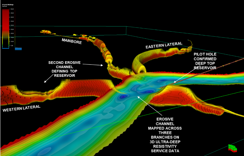
Particular focus for these investigations has been on complex environments where lateral variation is expected and 1D inversion does not show the complete picture. One such example is turbidite deposition, where mass flow deposits can result in both erosion and rapid deposition with the potential for multiple mass flows. 3D inversion of a trilateral well, though one such example, shows the complexity of the reservoir and the benefits that 3D inversion can bring to reservoir understanding (Figure 3).
Conclusion
In complex geological environments and mature fields where production and water injection result in complex fluid movements, 3D inversion of ultradeep EM data provides a useful tool for identifying a change in resistivity all around the borehole. It provides a deeper reservoir understanding beyond the position of resistivity boundaries reported above and below the borehole from existing technologies. The significant distances away from the wellbore that changes can be identified allow well placement decisions to be made early and the potential to make azimuthal changes to the well path based on the evolving reservoir picture as well as changes to true vertical depth.
Recommended Reading

Daniel Berenbaum Joins Bloom Energy as CFO
2024-04-17 - Berenbaum succeeds CFO Greg Cameron, who is staying with Bloom until mid-May to facilitate the transition.
Equinor Releases Overview of Share Buyback Program
2024-04-17 - Equinor said the maximum shares to be repurchased is 16.8 million, of which up to 7.4 million shares can be acquired until May 15 and up to 9.4 million shares until Jan. 15, 2025 — the program’s end date.

Mexico Pacific Appoints New CEO Bairstow
2024-04-15 - Sarah Bairstow joined Mexico Pacific Ltd. in 2019 and is assuming the CEO role following Ivan Van der Walt’s resignation.
Global Partners Declares Cash Distribution for Series B Preferred Units
2024-04-15 - Global Partners LP announced a quarterly cash dividend on its 9.5% fixed-rate Series B preferred units

W&T Offshore Adds John D. Buchanan to Board
2024-04-12 - W&T Offshore’s appointment of John D. Buchanan brings the number of company directors to six.