Spectral decomposition of seismic data is widely used for analysis of subtle stratigraphic plays and fractured reservoirs. The seismic data are transformed from the time domain to the frequency domain to generate the spectral magnitude and phase components at every time sample within the seismic data bandwidth. The spectral magnitude and phase components are then interpreted at different frequencies, which is similar to interpreting the subsurface stratigraphic features at different scales. Alternative methods include the traditional Fourier transform, continuous wavelet transform, S-transform and matching pursuit workflows, each having its own limitations and merits.
Although introduced 20 years ago, the spectral voice components have rarely been used in the seismic industry. The voice components can be considered as band-pass-filtered versions of the seismic data. In the frequency domain, the bandpass filter for a given frequency, f, is defined by a Gaussian spectrum with mean μ=f and with standard deviation σ=f such that the bandwidth of the voice component increases as the frequencies increase from the lower end of the bandwidth to the higher end. The corresponding wavelet is called a Morlet wavelet.
Figure 1 shows a comparison of vertical sections from the input seismic data, its spectral magnitude at f=50 Hz and its corresponding voice component. Notice that the vertical discontinuity information is not clearly seen on the spectral magnitude since the amplitudes are similar on either side of the fault. Instead, the discontinuity information is contained in the 50-Hz phase component, which is sensitive to the vertical time shift in the reflection event. The voice component combines the magnitude and phase information and clearly shows the fault. This observation could be exploited by either interpreting the discontinuity information as such or by running discontinuity attributes such as coherence on the voice component volume.

Figure 2 shows a comparison of the coherence strat-slice displays computed from the broadband input seismic data and the narrow-band voice components at 65 Hz, 70 Hz and 75 Hz. Notice the clarity in the definition of the discontinuities of the voice components coherence displays. Such images provide a means of delineating subtle faults with small offset that might be overlooked on the input data. A drawback of this approach is that the interpreter now has multiple frequency volumes to interpret, increasing the interpretation workload.

Workload ease
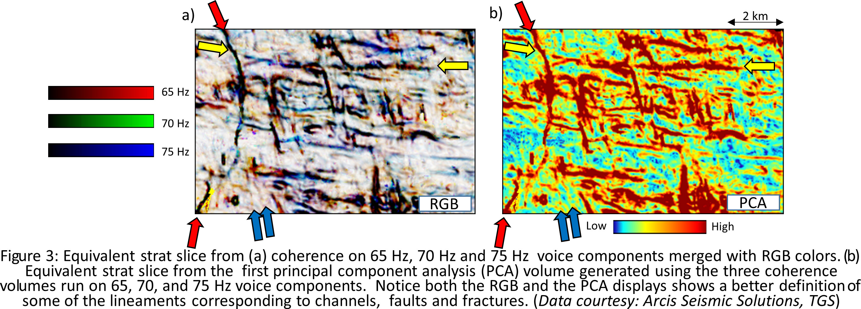
The most common use of spectral component magnitudes is to map stratigraphic objectives at or below the limits of seismic resolution on seismic stratal slices. Specifically, the time thickness of a channel often can be estimated to be T=1/(2fpeak), where fpeak is the frequency of the spectral component having the maximum magnitude. More complete information on seismic geomorphology can be gained by animating through a suite of frequency components or by combining three frequency components using an RGB color scheme. Figure 3a shows such a display, where the coherence attribute computed from the 65-Hz, 70-Hz and 75-Hz voices have been merged using red, green and blue (RGB) colors. By doing so, the detailed discontinuity information available in the three different attributes can be integrated into one display. Where the coherence anomaly appears on all three components, we get black. However, where the anomaly appears on only one component, we obtain the corresponding color. Finally, where the anomaly appears on two of the components, we obtain a cyan-, yellow- or magenta-blended color. Given this observation, note that anomalies that are absent in one of the components are “filled in” when plotted together using RGB.
While RGB color addition provides a means of graphically combining three components of information, principal component analysis provides a numerical means of achieving a similar result. Since the input volumes (the coherence images shown in Figures 2b-d) enhance structural edges, principal components will highlight the most important structural trends consistent in the three data volumes. Mathematically, the coherence volumes are cross-correlated with themselves and each other, forming a 3 by 3 covariance matrix. The first eigenvector of that matrix represents the linear combination of the three input attributes that best represent the energy variability of the three volumes. The first principal component is the correlation between this first eigenvector and the three values at each data sample (or voxel). For good-quality data, one would expect the same fault to be seen on closely spaced (60-Hz, 65-Hz and 70-Hz) voice components.
In this situation, the eigenvector simply tells us the relative amplitude of each frequency component’s coherence anomaly. If the variation of amplitude at a given discontinuity has this same proportion, which requires all three anomalies to line up, then the first principal component is a maximum. If one of the three anomalies is absent, the principal component will be lower. Finally, if the anomalies on the three components are random, which happens when noise contaminates the data, the principal
component will be small. Figure 3b displays the first principal component corresponding to the strat-slice shown in Figure 3a, computed from the coherence attributes computed from the 65-Hz, 70-Hz and 75-Hz voice components shown in Figures 2b-d. Notice that the principal component display has captured the same discontinuity information seen in Figure 3a. An important point to note here is that while the RGB integration can be carried out on just three different attributes, principal component analysis can be carried out on a number of input attributes. In this sense it is a much better dimensionality reduction tool.
Voice components derived from spectral decomposition of input seismic data furnish detailed and crisp information at specific frequencies that is amenable to more accurate interpretation. Discontinuity attributes such as coherence computed on such voice components help in making accurate interpretation of stratigraphic features, including faults and fractures.
Acknowledgements
The authors of this article thank Arcis Seismic Solutions, TGS, for encouraging this work and for permission to present these results.
Recommended Reading

TPG Adds Lebovitz as Head of Infrastructure for Climate Investing Platform
2024-02-07 - TPG Rise Climate was launched in 2021 to make investments across asset classes in climate solutions globally.

Sherrill to Lead HEP’s Low Carbon Solutions Division
2024-02-06 - Richard Sherill will serve as president of Howard Energy Partners’ low carbon solutions division, while also serving on Talos Energy’s board.

Magnolia Appoints David Khani to Board
2024-02-08 - David Khani’s appointment to Magnolia Oil & Gas’ board as an independent director brings the board’s size to eight members.

BP’s Kate Thomson Promoted to CFO, Joins Board
2024-02-05 - Before becoming BP’s interim CFO in September 2023, Kate Thomson served as senior vice president of finance for production and operations.

Magnolia Oil & Gas Hikes Quarterly Cash Dividend by 13%
2024-02-05 - Magnolia’s dividend will rise 13% to $0.13 per share, the company said.