The dramatic expansion in computing power and the huge amounts of data generated within organizations have led to an increase in new methods to identify patterns and trends among large datasets. Chief among these are data mining and predictive analytics (also called machine-learning processes)—cross-disciplinary approaches consisting of advanced computational statistics that are able to recognize patterns and predict trends from the data.
The healthcare, finance and retailing sectors (among many others) all rely on such methods and algorithms to extract information, correlations and interplays and to predict the behavior of systems.
Data mining and predictive analytics also can be applied to the upstream oil and gas industry. The result is a powerful tool for optimizing well planning and production.
What is predictive analytics?
Predictive analytics is a knowledge-based approach that uses automated pattern discovery and analyzes current behaviors to predict future outcomes. In other words, it relies on techniques that are able to learn from existing data properties.
A typical predictive analytics workflow often consists of two stages: gathering patterns from the data and deriving rules to identify underlying interplays and using known results to train a model against the available data with future results predicted by using these models.
Many algorithms are available today to identify correlations between data. The classification of these methods depends both on the nature of the learning process and on the desired output.
Supervised algorithms such as support vector machines or nearest neighbor algorithms are based on rules given by a user, which are adopted by the computer to map input into outputs, whereas unsupervised learning processes leave it to the computer to find the underlying data structure (cluster analysis).
Regression is another example of a supervised machine-learning process where the output is continuous rather than discrete. Classification processes are used to map outputs into discrete categories. Clustering techniques divide inputs into various groups based on the identification of hidden patterns. But unlike classifications where labels are known beforehand, groups are not known, which makes this process an unsupervised one.
The combination of data mining, which is used to explore existing data, and predictive analytics, which focuses on the predictive power of the algorithms, creates powerful methods to discover unknown areas of interest.
Identifying sweet spots
In unconventional reservoirs, sweet spot recognition is essential to reducing uncertainty, high-grading acreage and improving field economics. Identifying sweet spots, however, requires a detailed understanding of complex reservoir properties and how these influence the productivity of the wells. Inevitably, this involves large amounts of data, from the static (horizons and faults)
through to lithological properties and organic content.
Classical approaches to mapping out and predicting reservoir behavior tend to combine geophysics, geology and reservoir engineering to estimate reservoir properties, both at local and regional scales. This integrated approach can be improved even further thanks to predictive analytics specifically designed to get the best out of large input datasets.
The workflow
The sweet spot prediction workflow that takes place within the latest version of Emerson’s reservoir modeling software Roxar RMS 2013.1 consists of the analysis of measurements that classify samples into specific groups characterized by predictive patterns. The goal of the workflow is to predict the potential interest of areas that are located far from the wells by identifying sets of indicators that show clear trends that correlate with the best producing wells. These most relevant properties can be
used as a training pattern, and the classification of samples can be expanded to the entire target region by exploring the nearest neighborhood of each sample to classify all points according to their similarities.
Selecting the data
In selecting the data for the new workflow, relevant datasets can be log measurements, 3-D grid properties and seismic data. These data are integrated into one geomodel that can be divided into sub-areas depending on the global size of the studied area.
Production data also are valuable to the workflow, but their variations in time can sometimes make their integration complex. To avoid this, it can be useful to deal with the data by different stages, for example at the frack stages. Production data also can be translated into well properties, reflecting the productivity of each well across time and depth.
Building the 3-D geomodel
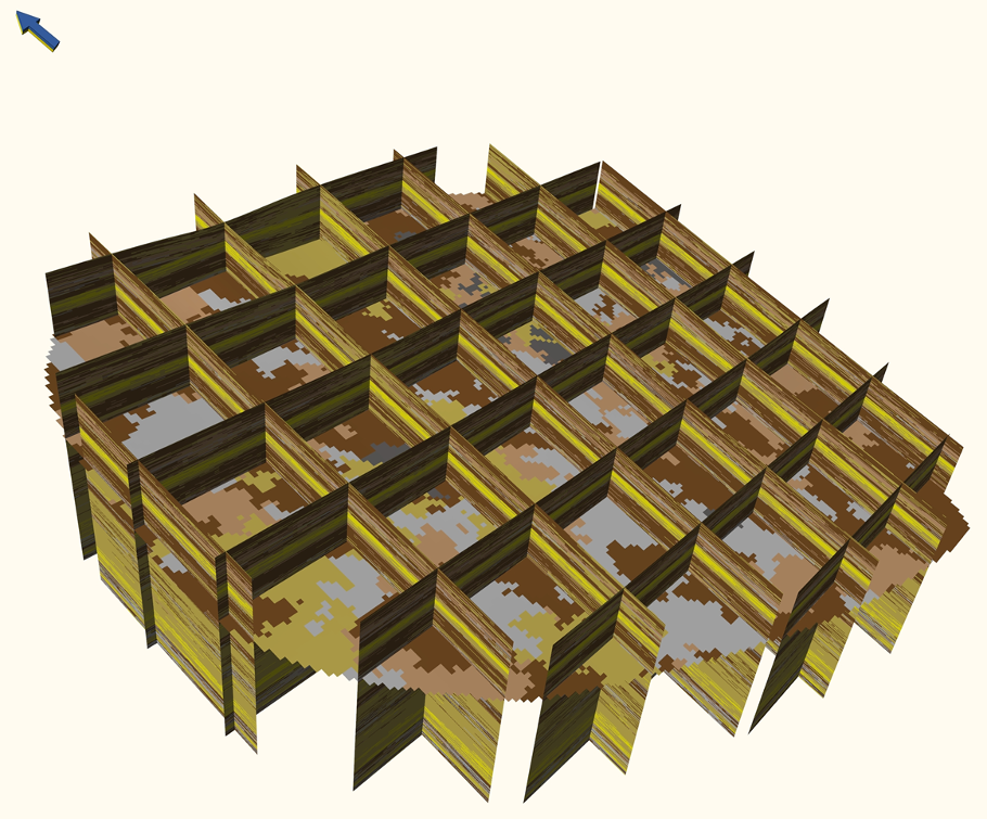
The 3-D geomodel can be built either in time or in depth, bringing together seismic interpretation, well correlation and properties modeling. This enables the kNN algorithm, a nearest neighbor classification algorithm, to be run on a full 3-D model, rendering both 3-D grid properties and average maps that show the location of potential sweet spots.
Filtering dependent properties beforehand also improves results, and the grid properties can then be used for volumes estimation and well planning. Figure 1 illustrates one such 3-D geomodel.
Source and nature of available data
In this example, measurements coming from the wells are wireline logs and petrophysical analysis. As part of the workflow, all well data are first quality-controlled to ensure that outliers don’t create unnecessary noise. The grid created from structural maps and limiting the reservoir areas is then populated with properties derived from both well data and seismic attributes.
Such properties include fracture density, rock brittleness, and gas saturation or thickness maps. In total, more than 15 properties have been used to generate the final model and maps in this example case.
Defining training dataset, applying algorithm
The next stage involves defining the training set and applying the classification algorithm. The classification process is based on user-defined selection, and the analytical toolbox available in Roxar RMS can be used to determine a reduced but optimal number of explanatory variables, including, for example, fracture density, total organic carbon and shale thickness. Working with a low number of explanatory variables makes the algorithm more robust and reduces the computational cost without sacrificing precision. Through the identification of similar patterns in areas with low well control, sweet-spot likelihood
maps can then be generated.
Potential sweet spots vs. nonsweet spots
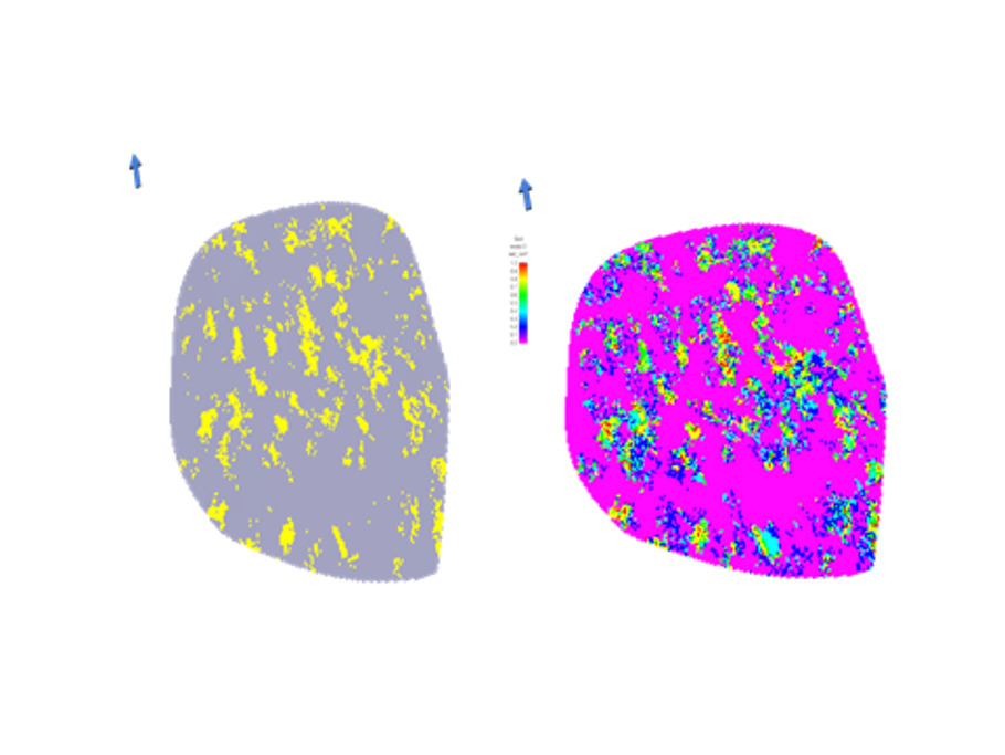
After the algorithm is run, the classification of the area of interest can be separated into two different classes: a potential sweet spot vs. a nonsweet spot.
The probability of the class to be correctly computed is then calculated, providing indications on the quality of the prediction. This is particularly important during risk assessment phases, in which several scenarios can be envisaged as a prelude to decision-making. Figure 2 illustrates this process.
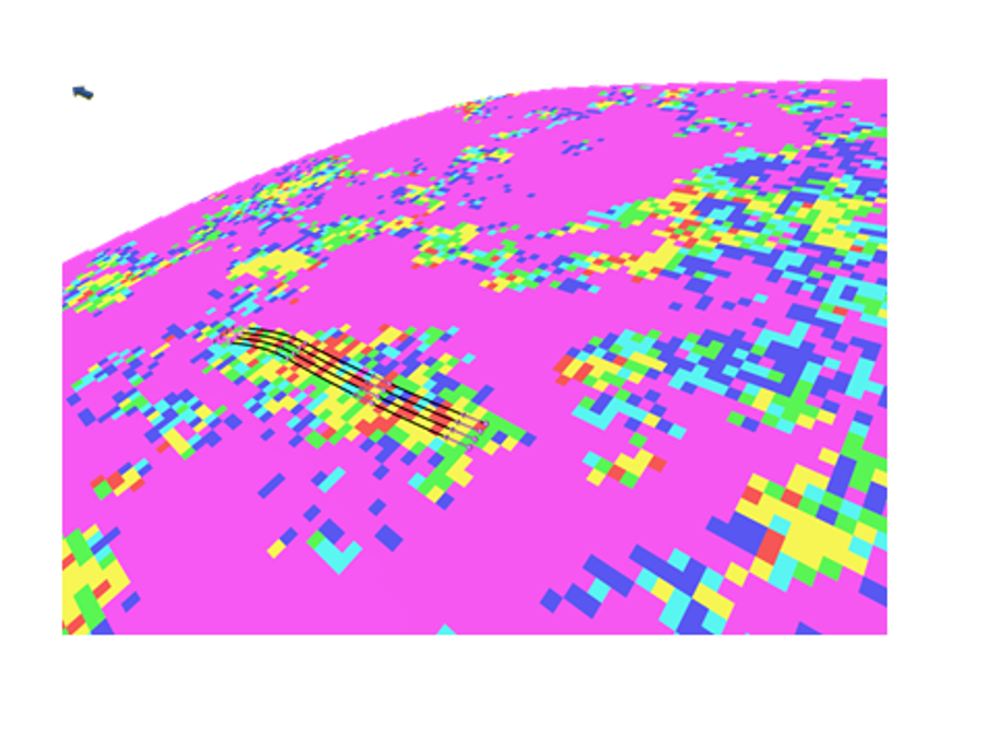
Once geologists and reservoir engineers have generated these maps, it is then possible to use them to plan new wells, predict production and even calibrate models using existing production history. Figure 3 illustrates future target locations. In addition, the likelihood parameter can play a key role in risk assessment and scenario ranking.
Through a step-by-step integrated and multidisciplinary workflow and the use of predictive analytic tools and machine-learning algorithms, datasets can be generated from unconventional reservoirs. They can be mined to their maximum potential to identify sweet spots and deliver improved decision-making on where to drill, what production strategies to adopt and how to unlock the value of operator assets.
In this way the relevance of geomodels can be enforced, classification algorithms can be used to capture complex interplays and predictive analytics can optimize unconventional reservoir investments.
Recommended Reading

Canada’s First FLNG Project Gets Underway
2024-04-12 - Black & Veatch and Samsung Heavy Industries have been given notice to proceed with a floating LNG facility near Kitimat, British Columbia, Canada.
Balticconnector Gas Pipeline Will be in Commercial Use Again April 22, Gasgrid Says
2024-04-17 - The Balticconnector subsea gas link between Estonia and Finland was damaged in October along with three telecoms cables.
Energy Transfer Asks FERC to Weigh in on Williams Gas Project
2024-04-08 - Energy Transfer's filing continues the dispute over Williams’ development of the Louisiana Energy Gateway.

Apollo Buys Out New Fortress Energy’s 20% Stake in LNG Firm Energos
2024-02-15 - New Fortress Energy will sell its 20% stake in Energos Infrastructure, created by the company and Apollo, but maintain charters with LNG vessels.

EQT CEO: Biden's LNG Pause Mirrors Midstream ‘Playbook’ of Delay, Doubt
2024-02-06 - At a Congressional hearing, EQT CEO Toby Rice blasted the Biden administration and said the same tactics used to stifle pipeline construction—by introducing delays and uncertainty—appear to be behind President Joe Biden’s pause on LNG terminal permitting.